how neural networks think at scale

Marmik Chaudhari, Nishkal Hundia

Introduction

Neural networks like Large Language Models (LLMs) first convert a sequence of input tokens into an $n$ dimensional vector by applying a linear transformation. This $n-$dimensional vector, called an embedding, then goes through a series of computations or layers like Attention and Multi Layer Perceptrons (MLP) and then is converted back into some output token by applying another linear transformation. These layers perform various linear and sometimes non-linear transformations on the embedding. The intermediate representations formed in the network at the end of each layer are called the hidden/ latent vectors or activations of the network.

The embedding passes through a series of transformations at each layer that extract or encode different kinds of information about the data in the activations. Mechanistic Interpretability (Mech Interp) aims at understanding these activations to reverse engineer how each component of the neural network cause it to produce a specific output. Since activations are high-dimensional vectors, the space of the possible activations is extremely large. This makes it unfeasible to explicitly visualize or analyze (the curse of dimensionality). So how do you understand them? By decomposing activations into independent understandable properties of the data, we can attribute different behaviors of the neural network to specific components. These properties of the data can also be thought of as interpretable “concepts”.

Most real world data has some structure. For instance, the color blue exists in the context of blue things like the sky or water, and words like 'king' and 'queen' share relational properties with 'man' and 'woman.' This occurs because concepts exist in relation to our understanding of other concepts. Language is built from finite vocabulary, has grammar rules, and syntactic structure. Images are composed of visual structures like edges, lines and objects. While low-level visual elements like edges and lines may not seem inherently meaningful on their own, they combine to form recognizable objects, textures, and patterns that do carry semantic meaning. We can think of this structure in terms of the interpretable "concepts"— meaningful ideas that capture important aspects of the data. While one could come up with an infinite number of such concepts, practically, a dataset can be represented by using a finite number of such concepts, say $k$. Furthermore, any reasonable input to the neural network makes use of a very small number of these interpretable concepts compared to the total number of available concepts, which makes the problem of decomposing the activations tractable.

While decomposability is necessary to solve the curse of dimensionality, we also need to be able to access the decomposition somehow. How do we find and extract these concepts from activation vectors? Linear representation of the concepts allows us to do this by determining which directions in the $n$-dimensional space correspond to which independent concepts of the input.

The Geometry of Embeddings

In order to decompose the activations of the neural network, one would want to understand the basis dimensions of its vector space.

The first transformation that an input to a LLM goes through is the word embedding. The vector space of word embeddings is rotational invariant. What does this mean in practical terms?Suppose $x$ is the word embedding of a particular word and let $W$ be the weight of the embedding matrix such that the $\mathrm{output} =Wx$. If you apply a linear transformation $M$ to the word embedding and apply $M^{-1}$ to the weight matrix, $W$, it will result in an identical model but where the basis dimensions are totally different. So, $x'= Mx$ and $W'= WM^{-1}$.

This demonstrates that the model’s computations are invariant to a change in its basis. In other words, the specific coordinates of the embeddings, or how they are represented in any particular basis, do not matter. What does matter is the relative geometry: how vectors relate to each other through directions, angles, and distances. This leads to a key insight about word embeddings: their space has no privileged basis. There is no “correct” or “canonical” set of axes in which to interpret them. This allows arithmetic like

and to define a “gender” direction by doing

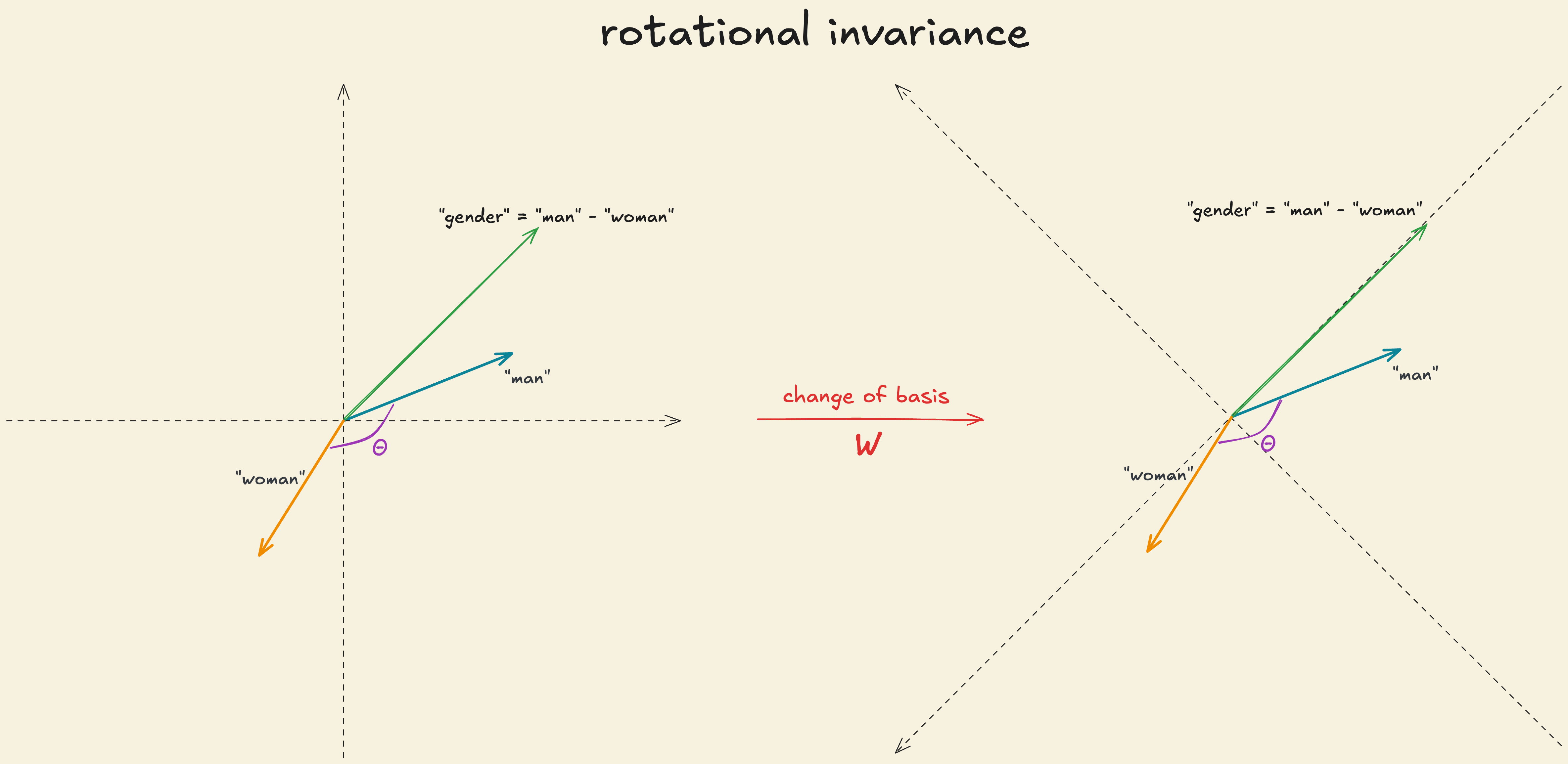
There’s no special relationship between the basis dimension and meaningful concepts. The interpretable concepts are embedded along any arbitrary direction in the vector space, making it non-privileged. In transformers, the residual stream and the attention vectors are non-privileged as well.

Basis of the Activation Space

In contrast, the vector space formed by a network layer’s activations is not like this. It is called the “representation” or activation space.

Consider an MLP that takes a flattened image input vector $x \in \mathbb{R}^n$ and produces an output $y \in \mathbb{R}^m$. Then, the activation vector is given by $h = Wx +b$ and the output $y=\text{ReLU}(h)$ where $W \in \mathbb{R}^{m\times n}$, $b \in \mathbb{R}^m$ and $\text{ReLU}$ is applied element-wise.

For the sake of simplicity, let’s also assume that the number of independent interpretable concepts, $k$, is equal to the dimensions of the activation space, $m$, meaning each basis dimension or coordinate, $h_i$, of the activation vector “captures” or detects one of the $k$ interpretable concepts. Consider that input vector $x$ represents a “yellow car”. The activation vector obtained after applying $W$ can be represented as,

after applying $\text{ReLU}$ element-wise,

The activation functions like $\text{ReLU}$ essentially “break the symmetry” as observed in word embeddings making certain dimensions more “special”. Since $\text{ReLU}$ operates independently on each coordinate, it introduces a preference for certain directions by only accepting positive parts of each dimension. Therefore, $\text{ReLU}$ gives each coordinate a distinct role: whether a neuron activates depends on how much the input projects along that specific axis. This makes the basis privileged: the default coordinate axes matter to the function of the network.

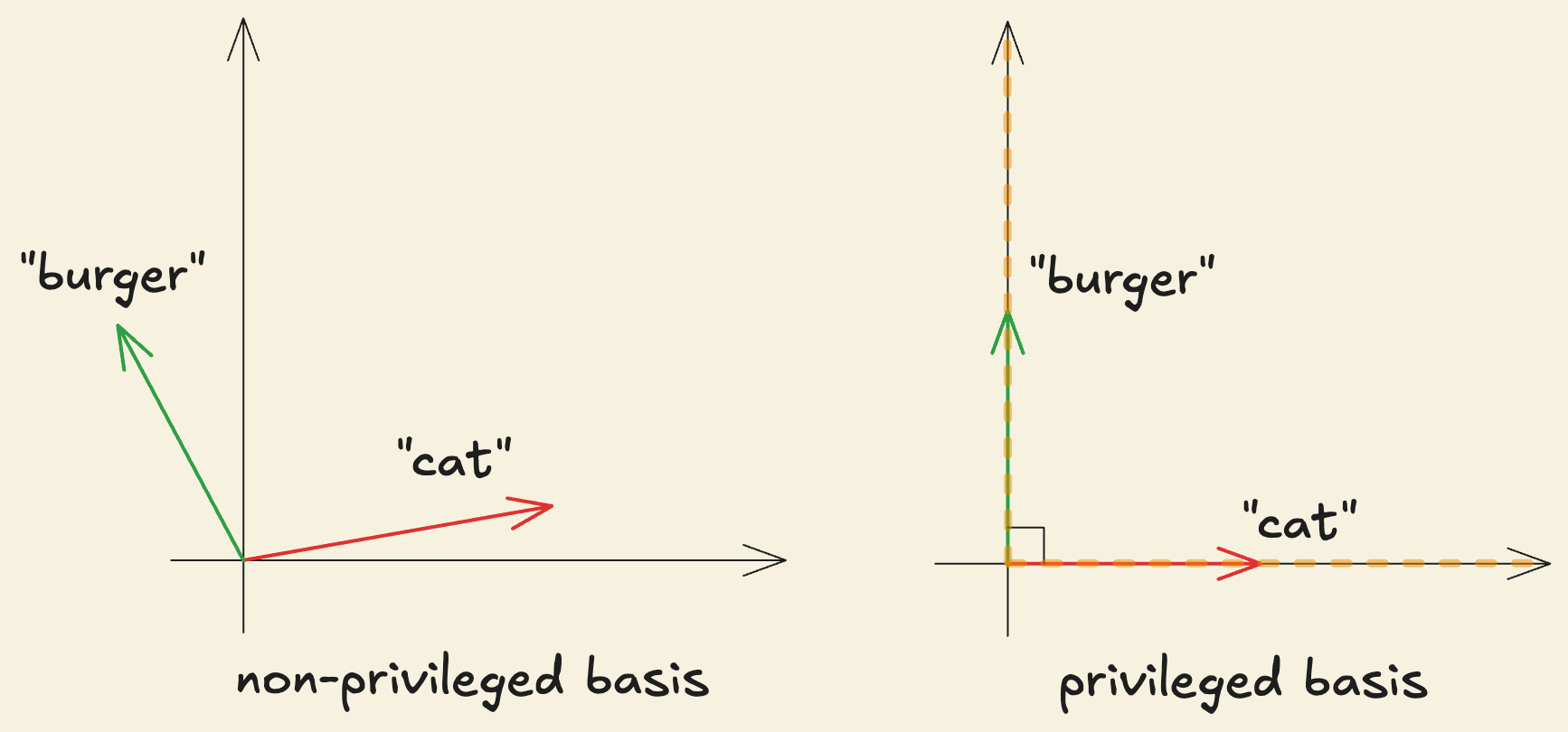
The dimensions of the activation space with privileged basis, i.e. the unique basis directions, are called “neurons”. The term neuron means that each basis dimension behaves like an independent computational unit that can respond to or detect specific interpretable concepts such as the “car shape” or the “yellow color”. From our MLP setup, each row of $W$acts like a template that tries to match a specific interpretable concept. Let’s say $W_3$ is the row vector corresponding to neuron 3 and is a “car shape” detector. The output of the neuron 3, given by $W_3 \cdot x$, would be non-zero after $\text{ReLU}$, indicating strong alignment between $W_3$ and $x$. We call this neuron “active”.

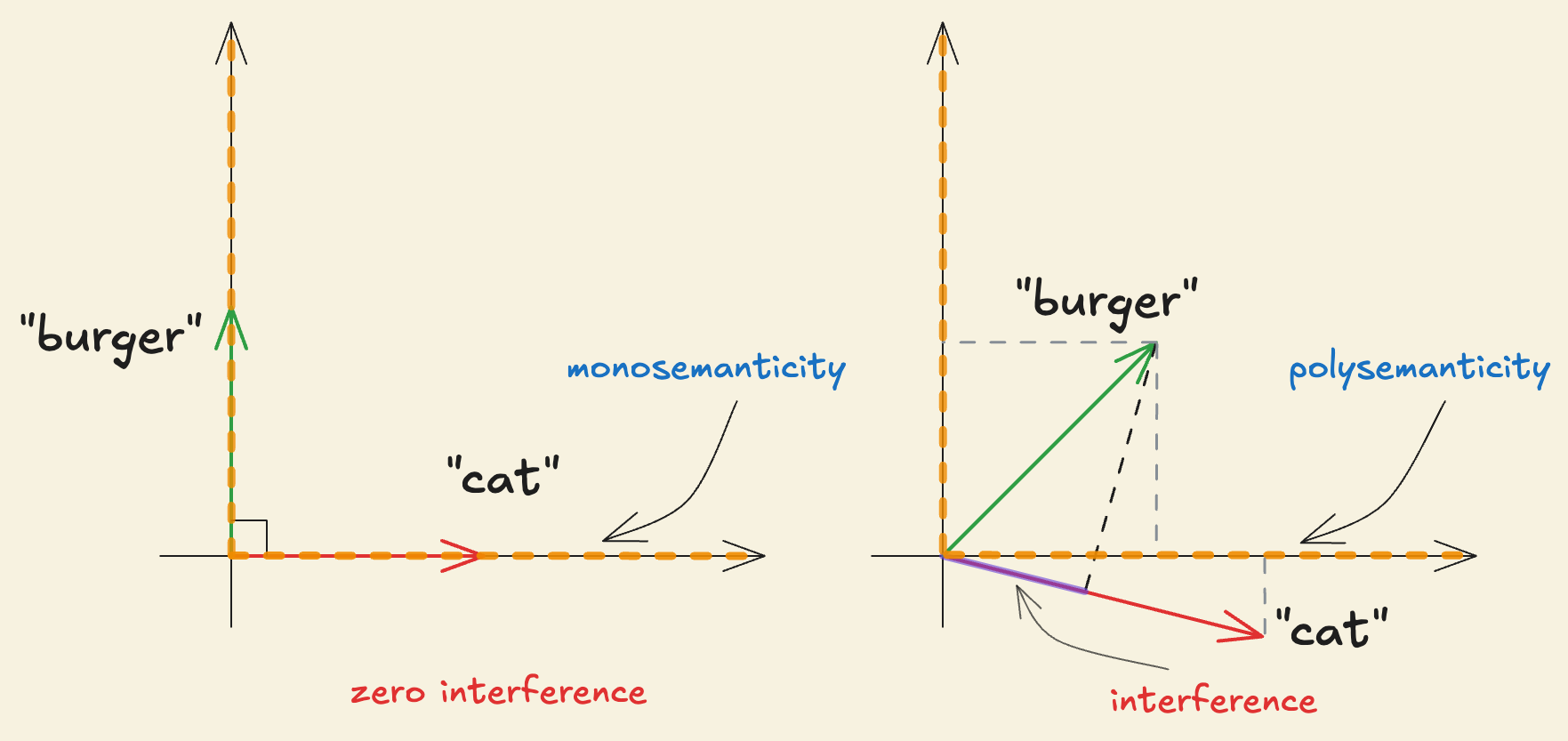
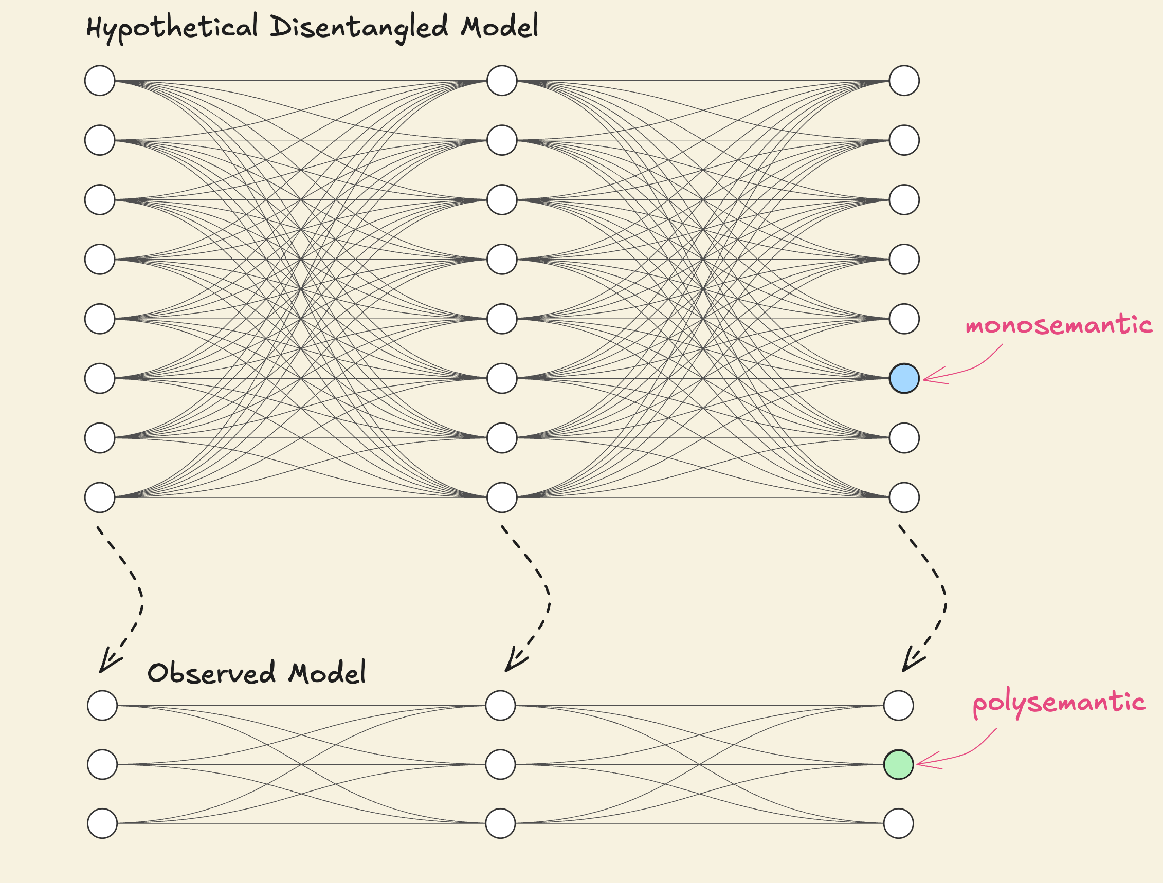
When individual neurons or the basis directions cleanly correspond to a specific interpretable concept, they are called monosemantic. But often, a single neuron is found to be responding to several unrelated but individually interpretable concepts, such as a neuron which responds to cat heads, car shapes, and jesus. Neurons that have grouped several unrelated interpretable concepts together are called polysemantic.

This raises the question of whether neurons — or more generally, the basis directions of the representation space — are the right framework to decompose activations and reason about interpretable concepts, given their polysemantic nature.

The Building Blocks

To address polysemanticity, we need a general abstraction for any interpretable direction in the activation space not necessarily aligned with any single neuron or basis direction. The directions in the activation space that correspond to an interpretable concept or an articulable property of the input such as car shape, dog head, edges are called features. Features can be thought of as being analogous to atoms in molecules. They represent the basic building block from which all neural network representations are constructed. Alternatively, a feature $f_i$ can also be defined as an arbitrary function of the input mapping $f_i : \mathcal{X} \rightarrow \mathbb{R}$ where $\mathcal{X}$ is the input (e.g, images, text) and $f_i(\mathbf{x})$ gives the “strength” or “presence” of feature $i$ in input $\mathbf{x}$. For example, a “car shape” feature would output high values for images with cars and low values otherwise.

But how do these “features” combine to produce the activation vector we observe?

For each of the $k$ interpretable concepts or features in the data, denoted by $f_1, f_2, f_3,…, f_k$, there exists a corresponding direction in the activation space, represented as $w_{f_1}, w_{f_2},…, w_{f_k} \in \mathbb{R}^n$. When a neural network processes a specific input, not all features are equally relevant or present. For example, an image might only contain edges and a car shape but no text or a dog head. Each feature $f_i$ has an activation strength associated with it, called “feature activation” , and is denoted by $x_{f_i} \in \mathbb{R}$ which represents “how much” of a particular concept is expressed in any given input and is a function of the input, $f_i(x)$. For example, an image with multiple cars would have high activation value for “car shape” features but near-zero activation for “dog-head” features.

Since features are defined as directions in the activation space, decomposing the activations in terms of these features makes the activations themselves linear. Thus, we define a linear representation hypothesis for neural network activations in terms of features: “Any activation vector, $h$ for an input containing multiple features, $f_i$ with feature activations, $x_{f_i}$ can be expressed as a linear combination of its feature directions, $w_{f_i}$”. Mathematically,

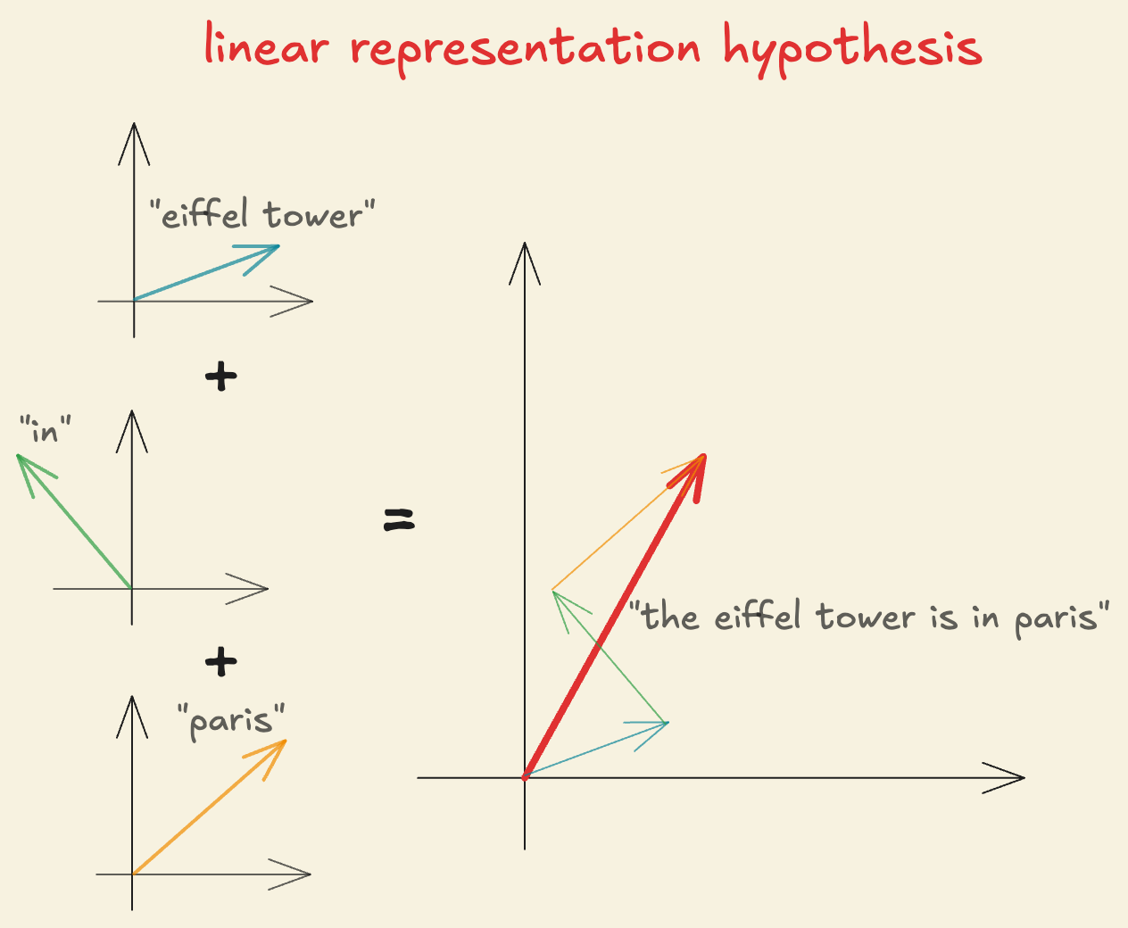
This provides a connection between defining features as both directions in the activation space and as a function of the input. It is also important to note that the process of extracting or representing the presence of features, $f_i(x)$ is non-linear. But once the feature activations are calculated, they are combined linearly to form the activation vector.

A natural question to ask is why should we expect the linear representation hypothesis to be true given that neural networks have non-linear functions like $\text{ReLU}$ and $\text{softmax}$ acting on the activations at various layers.

Neural networks are built with linear functions along with some non-linearities. But the majority of the computations inside a neural network are linear functions (scales $O(d^2)$ due to matrix-matrix multiply) while the non-linearity comprises of a very small part of the entire computation (scales $O(d)$ since its element-wise) (in FLOPs).

More importantly for understanding neural networks, linear representations have some key benefits:

• Each neuron can be thought of as detecting a specific pattern by taking the dot product of the input, $\mathbf{x}$, with its weight vector, $\mathbf{w}$, and gives an activation score. If the neuron is detecting feature $f_i$ then the activation, $\mathbf{w} \cdot \mathbf{x}$ varies linearly with the strength of the feature $f_i$. The dot product provides a natural way to do such “pattern” matching.

• If the activation of a previous layer, $\ell$ is represented linearly by $\mathbf{h}^{(\ell)} = \sum_{i=1}^{k} x_{f_i} \cdot \mathbf{w}_{f_i}$ and the pre-activation value of a neuron in the next layer, $\ell +1$ is defined as $z_j^{(\ell+1)} = \mathbf{w}_j^{(\ell+1)} \cdot \mathbf{h}^{(\ell)}$ then substituting $\mathbf{h}^{(\ell)}$ in the pre-activation,

  $$z_j^{(\ell+1)} = \mathbf{w}_j^{(\ell+1)} \cdot \left( \sum_{i=1}^{k} x_{f_i} \cdot \mathbf{w}_{f_i} \right) = \sum_{i=1}^{k} x_{f_i} \cdot (\mathbf{w}_j^{(\ell+1)} \cdot \mathbf{w}_{f_i})$$

  where $\mathbf{w}_j^{(\ell+1)} \cdot \mathbf{w}_{f_i}$ represents the alignment between neuron $j$ and feature $f_i$. This allows the neuron to selectively respond to any individual or combination of features in a single computational step making the features “linearly accessible”. If a feature was represented non-linearly, then the model would not be able to do it in a single step.

• Representing features as directions also allows for non-local generalization, for example, if you learn that features $A$ and $B$ combine to produce output $y$, you can immediately generalize to any new combination of features $A$ and $B$ even if you’ve never seen that exact combination before.

Furthermore, monosemantic neurons can be thought of as special cases of features as directions in the representation where it perfectly aligns with a privileged basis direction in the representation, i.e. $\mathbf{w}_{f_i} = \mathbf{e}_{f_i}$ where $\mathbf{e}_{f_i}$ is the standard basis vector of feature $f_i$. The activation vector $\mathbf{h}$ can be then represented as,

The decomposition of the activation vector in this case is trivial as each coordinate $h_i$ directly tells us the activation strength of feature $f_i$. For example, the decomposition of an activation vector representing “dog-head” would then look like $\mathbf{h}_{\text{dog head}} = 0.8 \cdot \mathbf{e}_{\text{floppy ear}} + 0.6 \cdot \mathbf{e}_{\text{golden fur}} + 0.9 \cdot \mathbf{e}_{\text{snout}} + \cdots$

A privileged basis is a necessary condition for interpretable neurons. Without it there’s no reason to expect any particular direction to be special. However, it doesn’t guarantee that features will be aligned with a privileged basis direction. In real world data there are far more interpretable concepts than neurons: $k >> n$, so most features cannot be aligned with the privileged basis directions. You can only have at most $n$ orthogonal directions in an $n$-dimensional space. The neural network faces an interesting choice during training: either represent the most important features monosemantically (aligning with the privileged basis directions) and ignore the remaining $k-n$ features, or represent more than $n$ features by sharing neurons, accepting some noise or interference.

Usually, a network chooses to pack multiple feature directions into a single neuron which results in neurons being polysemantic responding to several unrelated features. A natural follow-up to ask is whether neural networks can noisily represent more features than they have neurons.

The Superposition Hypothesis

Consider any two features $f_i$ and $f_j$ with their directions represented as $w_{f_i}$ , $w_{f_j} \in \mathbb{R}^n$ respectively. When multiple features are active simultaneously with activations $x_{f_1}, x_{f_2}, …, x_{f_k}$, the activation vector is $\mathbf{h} = \sum_{i=1}^{k} x_{f_i} \cdot \mathbf{w}_{f_i}$. The presence or activation of feature $f_j$ in $\mathbf{h}$ can be calculated as $x_{f_j} = \mathbf{h} \cdot \mathbf{w}_{f_j}$. So, $x_{f_j}$ can be rewritten as,

The term $(\mathbf{w}_{f_i} \cdot \mathbf{w}_{f_j})$ measures how aligned feature direction $\mathbf{w}_{f_i}$ is with $\mathbf{w}_{f_j}$. For a neuron to be monosemantic and represent feature $f_i$, we need $\mathbf{w}_{f_i} \cdot \mathbf{w}_{f_j} = 0 \quad \text{for all } i \ne j$ (be orthogonal to every other feature direction) and $\mathbf{w}_{f_i} \cdot \mathbf{w}_{f_i} = 1$ . Since $k > n$, we cannot make all feature directions $w_{f_i}$ and $w_{f_j}$ orthogonal, meaning that for certain feature pairs $f_i$ and $f_j$ where $i \ne j$, $\mathbf{w}_{f_i} \cdot \mathbf{w}_{f_j} \ne 0$. Now, the activation of feature $f_j$ becomes,

Furthermore, say for a particular input only feature $f_i$ is actually present with $x_{f_i} > 0$ and $f_j$ is not present ($x_{f_j} = 0$), then

This creates the interference problem where, when feature $f_i$ activates with $x_{f_i}$, it causes feature $f_j$ to activate even when $x_{f_j} =0$ since $f_j$ and $f_i$ are not orthogonal. When $k>n$, the term $(\mathbf{w}_{f_i} \cdot \mathbf{w}_{f_j})$ represents interference that feature $f_i$ causes in the direction of feature $f_j$. The interference problem seems to suggest that representing $k>n$ features in a $n$-dimensional space is sub-optimal due to the unavoidable “false” activation between non-orthogonal directions.

However, neural networks have been found to represent far more features than they have neurons. For example, a vision model with thousands of neurons can effectively represent millions of objects and visual patterns and language models with finite neurons also demonstrate a vast amount of knowledge.

Neural networks exploit a powerful property of high-dimensional spaces to represent far more features than they have neurons. According to the Johnson-Lindenstrauss Lemma, for some small $\epsilon > 0$, and any number of features $k$, if $n$ is sufficiently large, specifically $n \geq C \cdot \frac{\log k}{\epsilon^2}$ for some constant $C$, there exists a set of $k$ unit vectors $\mathbf{w}_{f_1}, \mathbf{w}_{f_2}, …,\mathbf{w}_{f_k}$ in $\mathbb{R}^n$ such that for all $i \neq j$

Tolerating a small amount of noise or interference allows the network to have $\text{exp}(n)$ many “almost orthogonal” vectors in high-dimensional spaces. Furthermore,

So, the number of features grows exponentially with the number of dimensions. With almost-orthogonal vectors, the interference terms become bounded as

But why do $n$-dimensional spaces have this property?

Let $\mathbf{u}, \mathbf{v}$ be two random unit vectors in $\mathbb{R}^n$ and their dot product is $\mathbf{u} \cdot \mathbf{v} = \sum_{i=1}^{n} u_i v_i$ and $\|\mathbf{u}\|^2 = u_1^2 + u_2^2 + \dots + u_n^2 = 1$. This means as $n$ increases, each individual component $u_i$ and $v_i$ gets smaller on average by $1/\sqrt{n}$ and the product $u_iv_i$ becomes even smaller (by $1/n$). Since $\mathbf{u}, \mathbf{v}$ are sampled randomly, $u_iv_i$ can be positive or negative with roughly equal probability. The sum of $u_iv_i$ over $n$ components cancels out roughly with very small remaining terms, $\mathbf{u} \cdot \mathbf{v} \approx 0$, making $\mathbf{u}$ and $\mathbf{v}$ almost orthogonal. High-dimensional spaces allow us to extend this phenomena from two nearly orthogonal vectors to exponentially many. When we add more vectors to our space, each new vector eliminates a very small fraction of the space. This allows us to have exponentially many almost-orthogonal vectors.

In language or vision models, the text or image data might contain millions of possible entities like “Martin Luther King”, “Shakespeare”, “Tokyo” or visual properties like “dog head”, “car wheels”, etc., but in any specific text or image input, only a very small fraction of all possible features are actually active. Most types of text or image input don’t talk about “Martin Luther King” or “dog head”. This means that feature are sparse, i.e. rarely active. Most interference terms vanish, as most features have activations $x_{f_i}=0$ and the sum is over a smaller subset of active features given by, $x_{f_j} = x_{f_j} + \sum_{i \in \text{ active features}} x_{f_i} \left( \mathbf{w}_{f_i} \cdot \mathbf{w}_{f_j} \right)$. This reduces the interference cost significantly.

Furthermore, different features affect the model’s performance or loss differently. A typical language model’s loss is given as $\mathcal{L}_{\text{prediction}} = -\log P(\text{next token} \mid \text{previous context})$. There are millions of features in data but some of them drive the loss down more than others. For example, when the input text contains Obama, having a “Barack Obama” feature dramatically narrows down the context and makes it easier to predict the next token by constraining the vocabulary and reducing uncertainty rather than, say, having a generic “middle name” feature. The “Barack Obama” feature heavily influences the text around it. Having core linguistic features like “verbs”, “adjectives” and “digits” is also crucial since most of the inputs make use of these concepts and it is important for the network to represent them efficiently to get strong performance (or low loss) and make next token prediction easier. On the other hand, most input text or image is not about “a specific person’s middle name” or “specific breed of dog”. Thus, these features rarely impact the network’s performance and are not as important as the “verbs” or “adjectives” features. This implies that features vary in importance.

Sparsity and feature importance allow neural networks to represent more features than they have neurons by exploiting the property of high-dimensional spaces discussed above. The presence of many sparse features in the underlying data dramatically reduces the interference cost. Feature importance introduces a hierarchy that guides which features of the input to represent and how much interference to tolerate for less important features. This helps the network represent many more important concepts moderately well, achieving lower loss than if it only represented the top $n$ features perfectly (orthogonally). Together, it makes superposition, “representing more feature than neurons”, an optimal strategy.

Concretely, the superposition hypothesis details how features are represented as almost orthogonal directions in the activation space. This, in turn, means that one feature activating looks like other features slightly activating (interference). The hypothesis also implies that especially important features might get dedicated neurons or almost orthogonal directions, making them monosemantic. For example, in vision models like Inception V1, critically important features like “curve detectors” or “high-low frequency detectors” have been seen to get dedicated neurons. The rest of the features that have categorically less importance may need to share the activation space and may not align with a specific neuron, making them polysemantic.

One alternate way to think about the superposition hypothesis is that a neural network is effectively a “compressed, noisy” version of a much larger, idealized network. In this hypothetical larger network, each neuron would correspond to exactly one of the infinite interpretable features with zero interference between features, creating a perfectly disentangled representation where every feature has its own dedicated dimension. However, the actual network we observe is a low-dimensional projection of the larger idealized network where the idealized neurons are projected on to the actual network as “almost orthogonal” vectors which, from the perspective of neurons, presents as polysemanticity.

The Challenges of Superposition

In a world with no superposition, we would have one-to-one correspondence between neurons and features and each feature $f_i$ would be represented by an orthogonal direction $\mathbf{w}_{f_i}$ which perfectly aligns with the basis direction $\mathbf{e}_{i}$.

With superposition, our activation vector becomes $\mathbf{h} = \sum_{i=1}^{k} x_{f_i} \cdot \mathbf{w}_{f_i}$ where the feature directions, $\mathbf{w}_{f_i}$’s are not orthogonal or basis aligned. One might try taking the dot product of the activation vector, $\mathbf{h}$ with feature direction $\mathbf{w}_{f_j}$ to get the activation strength as

But the activation strength contains other interference terms from all other active features and becomes misleading. We cannot decompose the activations in terms of pure features which obstructs the fundamental goal of mech interp.

Secondly, to confidently attribute certain behaviors, like deception or manipulation, to a model (or confirm their absence), we need the ability to identify and enumerate over all features it represents. This provides us with a universal quantifier over the fundamental units of a neural network. Without superposition in a privileged basis, enumerating over features would be as simple as enumerating over neurons since each neuron would represent a feature. However, with superposition, the number of features that exist in the activation space is unknown due to polysemantic neurons. This obstructs the ability to enumerate over the features.

solutions

The connection between superposition and enumerating features also goes the other way. If we’re somehow able to enumerate over features, one can “unfold” a superposed model’s activations into those of a larger, non-superposed model.

If we have an activation vector $\mathbf{h} \in \mathbb{R}^n$ that represents a compressed combination of $k>n$ features, then how can you “un-compress” it back to identify which features are active? There are $k$ unknowns but only $n$ equations which is an underdetermined system. Such systems have infinitely many equations and the solutions aren’t unique. For example, for the equation $x+y+z=6$, there’s no way for us to recover $x=2,y=3,z=1$ as $x=4,y=1,z=1$ can work as well.

But the problem becomes tractable if your features are sparse. In this case, it is possible to recover the original vector or constituents. For $k$ features, the map from the feature activation vector, $\mathbf{x} = \begin{bmatrix} x_1, x_2, \ldots, x_k \end{bmatrix}^T \in \mathbb{R}^k$ to $n$ neurons as in the network given by, $\mathbf{h} \in \mathbb{R}^n$ can be represented as

where $\mathbf{W} \in \mathbb{R}^{n\times k}$ is the feature direction matrix with each column $\mathbf{w}_i$ representing the direction of feature $i$.

This is a standard sparse coding or recovery problem. We want to learn an overcomplete set of basis vectors in the activation space, $\mathbf{w}_i$ to represent input vectors, $\mathbf{h} \in \mathbb{R}^n$ to recover the sparse feature activations, $x_i$. The advantage of having an overcomplete basis is that our basis vectors are better able to capture structure and patterns inherent in the input data. Furthermore, we introduce an additional criterion of sparsity to avoid having an infinite combination of feature activations or coefficients. The sparsity criterion puts the constraint of reconstructing the input vector using the fewest possible basis vectors and makes the solution unique.

Next, we want to minimize the “reconstruction error” which measures how well our decomposition reconstructs the original activation or input vector and is given as

Furthermore, we introduce an L1 sparsity penalty which encourages most of the feature activations, $x_i$ to be zero or close to zero and is written as

where $\lambda >0$ is the regularization parameter and controls the strength of the penalty.

Combining the reconstruction and sparsity error, the complete objective function for the sparse coding problem is

Since we don’t know either $\mathbf{W}$ or $\mathbf{x}$ initially, we perform a two step learning process. First involving learning the feature activations or coefficients, $x_i$ for some fixed feature directions, $\mathbf{W}$. Then we take the learned feature activations, $x_i$ and use them to optimize our feature directions with the objective function, $\min_{_\mathbf{W}} \sum_{j} \left\| \mathbf{h}^{(j)} - \mathbf{W} \mathbf{x}^{(j)} \right\|_2^2$ over $j$ training samples subject to $\left\| \mathbf{w}_i \right\|_2 = 1$ to keep the directions normalized.

Another approach to solving superposition involves simply applying a L1 regularization term to the hidden layer activations, i.e. add $\lambda \left\| \mathbf{h} \right\|_1$ to the loss. Intuitively, it kills the features that are below a certain importance threshold, especially if they’re not basis aligned. Getting rid of superposition with such penalty may be fairly achievable but comes at a large performance cost. Notably, superposition seems to significantly benefit neural networks, effectively making the networks much bigger.

Looking ahead

Even though past work demonstrating superposition, how it influences learning, and the geometry of the features in superposition exists, there still remain many open questions to answer. For example, should superposition just go away if we scale the network enough or is there a statistical test for catching superposition? Developing a deep understanding of how the models learn certain behaviors and how learning gives rise to its own world of structure and elegant complexity is an avenue worth exploring. It makes interpretability almost equivalent to the biology of artificial neural networks. We hope to have convinced you of the same.

Thanks to Rome Thorstenson, Benjamin Klieger, Jeremi Nuer, Swastik Agarwal, Pranav Karra, Idhant Gulati and Viraj Chhajed for providing valuable feedback on the draft.

References & Further reading

This work has been heavily inspired from the work on Toy Models of Superposition by Elhage et al. Here are some papers for further reading on related topics.

1. Olah, et al., "Zoom In: An Introduction to Circuits", Distill, 2020.

2. Gabriel Goh, “Decoding Thought Vector”.

3. Stanford UFLDL, “Sparse Coding”.

4. Cunningham, et al., “Sparse Autoencoders Find Highly Interpretable Features in Language Models”, ICLR, 2024.

5. Elhage, et al., "A Mathematical Framework for Transformer Circuits", Transformer Circuits Thread, 2021.

6. Lindsey, et al., "On the Biology of a Large Language Model", Transformer Circuits, 2025.

7. Bricken, et al., "Towards Monosemanticity: Decomposing Language Models With Dictionary Learning", Transformer Circuits Thread, 2023.